4: Macro and Micro Regions Analysis
Demonstrate the usage of SpatialCells to extract region components or holes for fine-grained analysis into cell types.
[11]:
import pandas as pd
import matplotlib.pyplot as plt
import anndata as ad
import seaborn as sns
import statistics
import spatialcells as spc
Read data
[3]:
adata = ad.read_h5ad("../../data/MEL1_adata.h5ad")
adata.obs["id"] = adata.obs_names
[4]:
adata.var_names
[4]:
Index(['SOX10_cellRingMask', 'KERATIN_cellRingMask', 'CD3D_cellRingMask',
       'MITF_cellRingMask', 'KI67_cellRingMask', 'CCND1_cellRingMask'],
      dtype='object')
setGate or setGates
This package relies on gated biomarkers in adata.obs
If gating has not yet been performed, setGate and setGates are convenience functions to gate the dataset manually or via a csv file
[6]:
spc.prep.setGate(adata, "SOX10_cellRingMask", 7.9, debug=True)
spc.prep.setGate(adata, "CCND1_cellRingMask", 7.5, debug=True)

adata.obs["CCND1_negative"] = ~adata.obs["CCND1_cellRingMask_positive"]
adata.obs["SOX10+CCND1-"] = adata.obs["SOX10_cellRingMask_positive"] & adata.obs["CCND1_negative"]
SOX10_cellRingMask_positive
False    566576
True     544009
Name: count, dtype: int64
CCND1_cellRingMask_positive
False    827121
True     283464
Name: count, dtype: int64
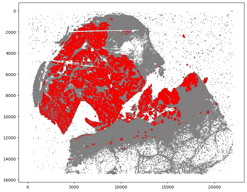
Visualizing cells with markers of interest
[7]:
fig, ax = plt.subplots(figsize=(10, 8))
ax.invert_yaxis()

## all points
ax.scatter(
    *zip(*adata.obs[["X_centroid", "Y_centroid"]].to_numpy()),
    s=1,
    color="grey",
    alpha=0.5
)
## SOX10+CCND1- cells
tmp = adata[adata.obs["SOX10+CCND1-"]]
ax.scatter(
    *zip(*tmp.obs[["X_centroid", "Y_centroid"]].to_numpy()),
    s=0.1,
    color="red",
    alpha=0.3
)
plt.show()
getCommunities
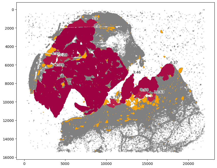
We first use DBSCAN via getCommunities to identify regions with high densities of markers of interest.
[15]:
markers_of_interest = ["SOX10+CCND1-"]
communitycolumn = "COI_community"
ret = spc.spatial.getCommunities(
    adata,
    markers_of_interest,
    eps=55,  # smaller --> more cells are considered as outliers.
    newcolumn=communitycolumn,
    min_samples=5,
    core_only=True,
)
print("number of communities:", len(ret[0]))
number of communities: 149
[16]:
help(spc.plt.plotCommunities)
Help on function plotCommunities in module spatialcells.plotting._plotCommunities:

plotCommunities(adata, ret, communitycolumn, plot_first_n_clusters=10, **kwargs)
    Plot largest communities on a scatter plot. Each community is labelled as:
    (rank in descending number of cells : index of community)

    :param adata: AnnData object
    :param ret: return value of spc.spa.getCommunities
    :param communitycolumn: column name of the community column in adata.obs
    :param plot_first_n_clusters: plot and number the largest n communities
    :param kwargs: keyword arguments for matplotlib.pyplot.plot
[17]:
fig, ax = plt.subplots(figsize=(10, 8))
spc.plt.plotCommunities(
    adata, ret, communitycolumn, plot_first_n_clusters=10, s=2, fontsize=10, ax=ax
)
ax.invert_yaxis()
plt.show()
[18]:
plot_first_n_clusters = 10
clusters_idx_sorted = [idx for npoints, idx in ret[0]]
print(
    "Indexes of the",
    plot_first_n_clusters,
    "largest clusters:\n",
    clusters_idx_sorted[:plot_first_n_clusters],
)
print("Cluster size and index:\n", ret[0][:plot_first_n_clusters])

# Here we choose the three largest ones of interest based on their index:
communityIndexList = [2, 8, 25, 28, 39]
Indexes of the 10 largest clusters:
 [8, 39, 46, 37, 2, 25, 28, 58, 76, 63]
Cluster size and index:
 [(165231, 8), (41772, 39), (29115, 46), (11021, 37), (7557, 2), (4439, 25), (3337, 28), (2560, 58), (1844, 76), (1778, 63)]
getBoundary
[19]:
help(spc.spatial.getBoundary)
Help on function getBoundary in module spatialcells.spatial._getBoundary:

getBoundary(anndata, communitycolumn, communityIndexList, alpha=100, debug=False)
    Get a boundary for the communities of interest as a Shapely MultiPolygon.

    The boundary is defined based on the alpha shape of points in the
    communities. The alpha shape is the generalization of the convex hull,
    and is generated via Delaunay triangulation of all the points of interest.
    The alpha parameter controls the longest edge that can appear in the alpha
    shape. Smaller alpha gives more detailed boundary, but may appear more
    jagged and may leave out some points that are too far away from the rest
    of the points.

    :param anndata: the anndata object
    :param communitycolumn: the column name of the community
    :param communityIndexList: the list of community indexes
    :param alpha: the alpha parameter for alpha shape. Smaller alpha gives
        more detailed boundary, but may appear more jagged.
    :param debug: whether to return the polygons and edge components
    :returns: the boundaries of components as a MultiPolygon object
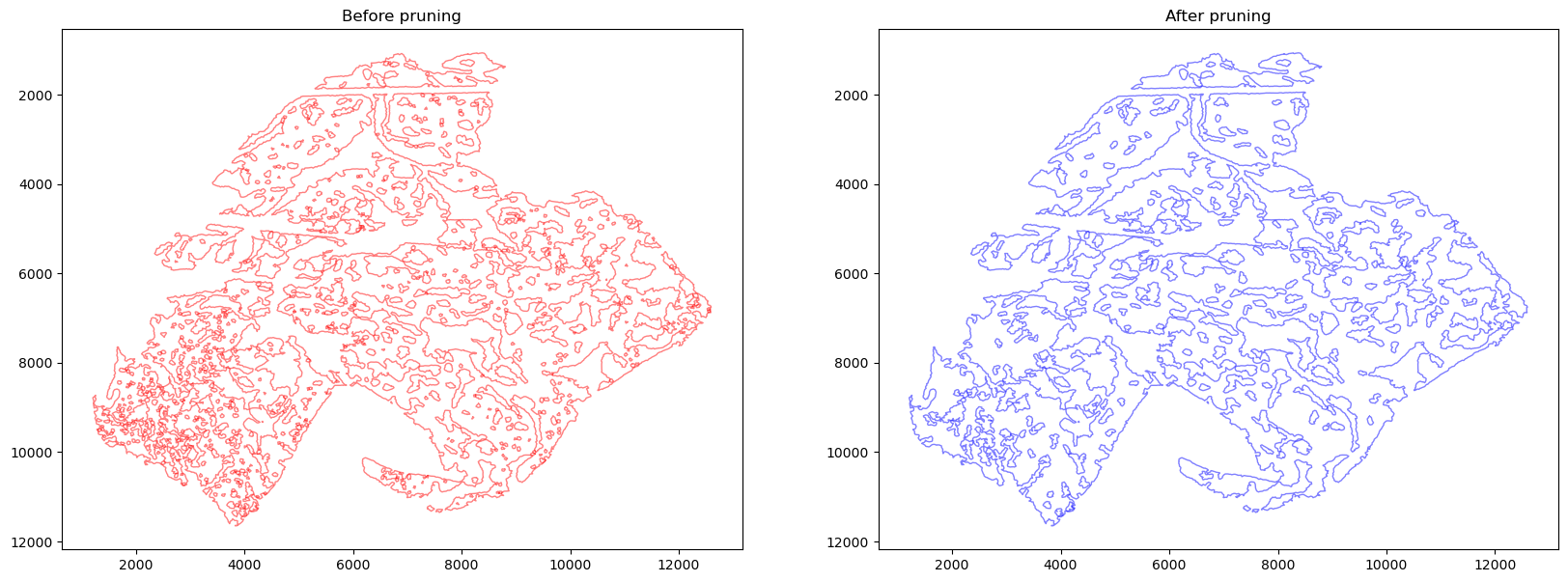
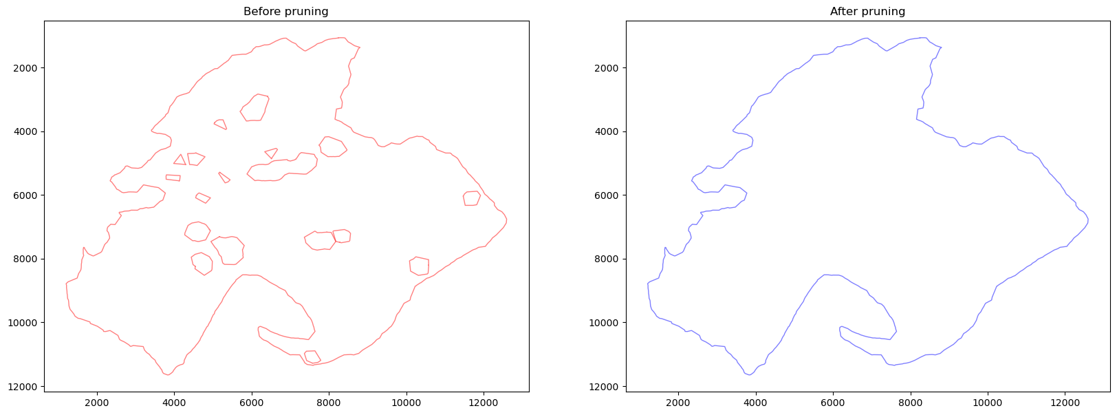
[20]:
# smaller alpha results in more detailed boundaries
boundaries, polygons, edge_components = spc.spatial.getBoundary(
    adata, communitycolumn, communityIndexList, alpha=27, debug=True
)
boundaries1 = spc.spatial.pruneSmallComponents(
    boundaries, min_area=0, min_edges=20, holes_min_area=10000, holes_min_edges=10
)
fig, [ax1, ax2] = plt.subplots(1, 2, figsize=(20, 7))
spc.plt.plotBoundary(boundaries, c="red", alpha=0.5, linewidth=1, ax=ax1)
spc.plt.plotBoundary(boundaries1, c="blue", alpha=0.5, linewidth=1, ax=ax2)
ax1.set_title("Before pruning")
ax2.set_title("After pruning")
ax1.invert_yaxis()
ax2.invert_yaxis()
plt.show()
Isolate and plot each boundary component (for demo)
[21]:
help(spc.spa.getComponents)
Help on function getComponents in module spatialcells.spatial._utils:

getComponents(boundary, keep_holes=True)
    Get the components of a boundary defined by a MultiPolygon.

    :param boundary: the boundary to get components from
    :param keep_holes: whether to keep holes
    :returns: a list of components, where each component is a MultiPolygon
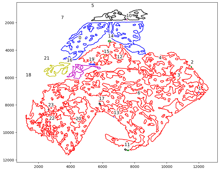
[22]:
boundary_component_list = spc.spa.getComponents(boundaries1)
print("Number of components:", len(boundary_component_list))
fig, ax = plt.subplots(figsize=(10, 8))
spc.plt.plotRegions(
    boundary_component_list,
    colors_list=["r", "b", "g", "y", "m", "k"],
    x_offset=0,
    y_offset=-200,
    ax=ax,
)
ax.invert_yaxis()
plt.show()
Number of components: 24
[23]:
# larger alpha results in more rough boundaries with less jagged exterior
boundaries_rough, polygons_rough, edge_components_rough = spc.spatial.getBoundary(
    adata, communitycolumn, communityIndexList, alpha=180, debug=True
)
boundaries_rough1 = spc.spatial.pruneSmallComponents(
    boundaries_rough,
    min_area=100000,
    min_edges=30,
    holes_min_area=4000,
    holes_min_edges=3000,
)
fig, [ax1, ax2] = plt.subplots(1, 2, figsize=(20, 7))
spc.plt.plotBoundary(boundaries_rough, c="red", alpha=0.5, linewidth=1, ax=ax1)
spc.plt.plotBoundary(boundaries_rough1, c="blue", alpha=0.5, linewidth=1, ax=ax2)
ax1.set_title("Before pruning")
ax2.set_title("After pruning")
ax1.invert_yaxis()
ax2.invert_yaxis()
plt.show()
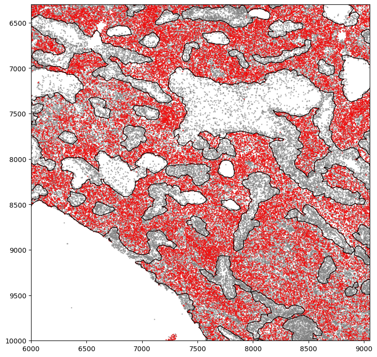
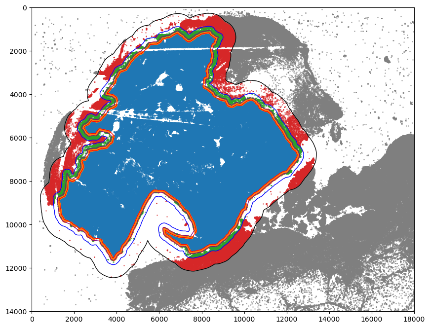
Visualization of regions of interest and boundary
[24]:
markersize = 1

fig, ax = plt.subplots(figsize=(9, 9))

## all points
ax.scatter(
    *zip(*adata.obs[["X_centroid", "Y_centroid"]].to_numpy()),
    s=markersize,
    color="grey",
    alpha=0.5,
    label="All cells"
)

# Points in selected commnities
xy = adata.obs[
    adata.obs["SOX10+CCND1-"]
][  # [adata.obs[communitycolumn].isin(communityIndexList)][
    ["X_centroid", "Y_centroid"]
].to_numpy()
ax.scatter(
    xy[:, 0],
    xy[:, 1],
    s=markersize,
    color="r",
    marker="o",
    alpha=0.5,
    label="SOX10+CCND1- cells",
)

# Bounds of points in selected commnities
spc.plt.plotBoundary(boundaries1, linewidth=1, color="k", ax=ax)
plt.ylim(6300, 10000)
plt.xlim(6000, 9050)
ax.invert_yaxis()
# plt.legend(loc="lower left", markerscale=5)
# plt.savefig("5_micro_region_zoom.png", dpi=300)
plt.show()
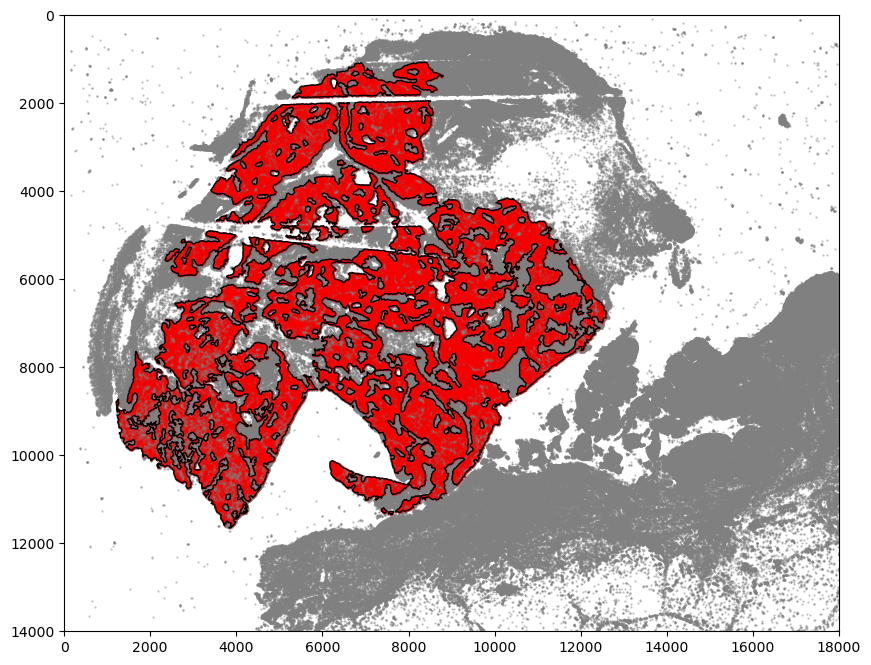
[25]:
markersize = 0.3

fig, ax = plt.subplots(figsize=(10, 8))

## all points
ax.scatter(
    *zip(*adata.obs[["X_centroid", "Y_centroid"]].to_numpy()),
    s=markersize,
    color="grey",
    alpha=0.5,
    label="All cells"
)

# Points in selected commnities
xy = adata.obs[
    adata.obs[communitycolumn].isin(communityIndexList)
][  # adata.obs[adata.obs["SOX10+CCND1-"]][
    ["X_centroid", "Y_centroid"]
].to_numpy()
ax.scatter(
    xy[:, 0],
    xy[:, 1],
    s=markersize,
    color="r",
    marker="o",
    alpha=0.2,
    label="SOX10+CCND1- cells",
)

# Bounds of points in selected commnities
spc.plt.plotBoundary(boundaries1, linewidth=1, color="k", ax=ax)
ax.invert_yaxis()
plt.ylim(14000, 0)
plt.xlim(0, 18000)
# plt.legend(loc="lower left", markerscale=5)
# plt.savefig("5_micro_region.png", dpi=300)
plt.show()
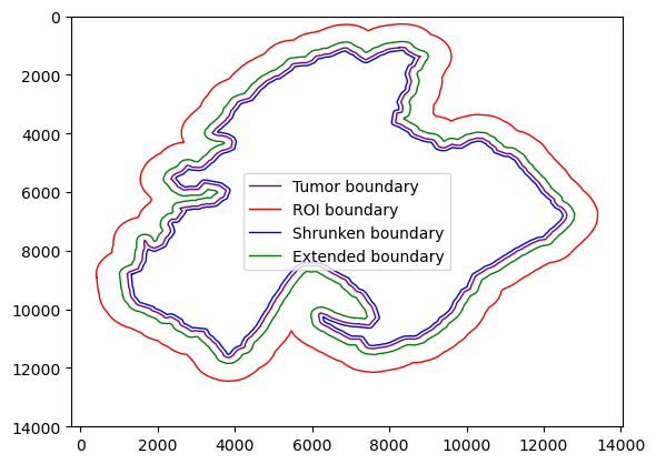
getExtendedBoundary & getShrunkenBoundary
getExtendedBoundary and getShrunkenBoundary can be used to expand or shrink the current boundary, which is useful to generate regions of interest
[26]:
shrunken_boundaries_rough = spc.spa.getShrunkenBoundary(boundaries_rough1, 100)
shrunken_boundaries_rough = spc.spatial.pruneSmallComponents(
    shrunken_boundaries_rough,
    min_area=0,
    min_edges=10,
    holes_min_area=1000,
    holes_min_edges=10,
)
extended_boundaries_rough = spc.spa.getExtendedBoundary(boundaries_rough1, 200)
extended_boundaries_rough = spc.spatial.pruneSmallComponents(
    extended_boundaries_rough,
    min_area=0,
    min_edges=10,
    holes_min_area=1000,
    holes_min_edges=10,
)
ROI_boundaries_rough = spc.spa.getExtendedBoundary(boundaries_rough1, 800)
ROI_boundaries_rough = spc.spatial.pruneSmallComponents(
    ROI_boundaries_rough,
    min_area=0,
    min_edges=20,
    holes_min_area=1000,
    holes_min_edges=10,
)

spc.plt.plotBoundary(
    boundaries_rough1, linewidth=1, color="purple", label="Tumor boundary"
)
spc.plt.plotBoundary(
    ROI_boundaries_rough, linewidth=1, color="red", label="ROI boundary"
)
spc.plt.plotBoundary(
    shrunken_boundaries_rough, linewidth=1, color="blue", label="Shrunken boundary"
)
spc.plt.plotBoundary(
    extended_boundaries_rough, linewidth=1, color="green", label="Extended boundary"
)
plt.ylim(14000, 0)
plt.legend(markerscale=5)
plt.show()
assignPointsToRegion
Using 1 or more generated boundaries, cells can be assigned to different regions for downstream analysis
[27]:
help(spc.spatial.assignPointsToRegions)
Help on function assignPointsToRegions in module spatialcells.spatial._assignPointsToRegions:

assignPointsToRegions(anndata, boundaries_list, region_names, assigncolumn='region', default='BG')
    Assign points to regions based on the boundaries. The region assignment is
    based on the order of the boundaries, so the innermost region should be the
    first element of boundaries_list.

    :param anndata: Anndata object
    :param boundaries_list: List of boundaries
    :param region_names: List of region names. The order and length should match boundaries_list
    :param assigncolumn: Column name for the region assignment
    :param default: Default region name for points that are not assigned to any region
[28]:
regions = ["Tumor", "Tumor Border", "Stroma Border", "Stroma"]
boundaries_list = [
    shrunken_boundaries_rough,
    boundaries_rough1,
    extended_boundaries_rough,
    ROI_boundaries_rough,
]
adata.obs["region_rough"] = "BG"
spc.spatial.assignPointsToRegions(
    adata, boundaries_list, regions, assigncolumn="region_rough", default="BG"
)
701940it [00:41, 17077.27it/s]
Assigned points to region: Tumor
184786it [00:11, 16340.51it/s]
Assigned points to region: Tumor Border
172844it [00:12, 13941.30it/s]
Assigned points to region: Stroma Border
227665it [00:10, 21396.41it/s]
Assigned points to region: Stroma
[29]:
print("Regions:")
print(adata.obs["region_rough"].cat.categories)
print("\nNumber of points in each region:")
print(adata.obs["region_rough"].value_counts())
Regions:
Index(['Tumor', 'Tumor Border', 'Stroma Border', 'Stroma', 'BG'], dtype='object')

Number of points in each region:
region_rough
Tumor            532328
BG               454981
Stroma            62020
Tumor Border      41576
Stroma Border     19680
Name: count, dtype: int64
[30]:
colors = ["tab:blue", "tab:orange", "tab:green", "tab:red", "tab:gray"]

point_size = 1
fig, ax = plt.subplots(figsize=(10, 8))

for i, region in enumerate(adata.obs["region_rough"].cat.categories):
    tmp = adata[adata.obs.region_rough == region]
    ax.scatter(
        *zip(*tmp.obs[["X_centroid", "Y_centroid"]].to_numpy()),
        s=point_size,
        alpha=0.5,
        label=region,
        color=colors[i]
    )

# Bounds of points in selected commnities
spc.plt.plotBoundary(
    boundaries_rough1, linewidth=1, color="purple", ax=ax, label="Tumor"
)
spc.plt.plotBoundary(ROI_boundaries_rough, linewidth=1, color="k", ax=ax, label="ROI")
spc.plt.plotBoundary(
    shrunken_boundaries_rough, linewidth=1, color="red", ax=ax, label="Shrunken tumor"
)
spc.plt.plotBoundary(
    extended_boundaries_rough, linewidth=1, color="blue", ax=ax, label="Extended tumor"
)
# plt.legend(loc="lower right", markerscale=5)
plt.ylim(14000, 0)
plt.xlim(0, 18000)
# plt.savefig("5_macro_regions.png", dpi=300)
plt.show()
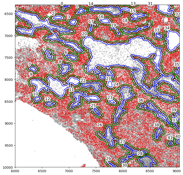
Isolate non-tumor cell holes within the tumor region:
[32]:
from shapely.geometry import Polygon

holes = spc.spa.getHoles(boundaries1)
final_holes = []
roi_poly = Polygon(
    [
        (6000, 10000),
        (9050, 10000),
        (9050, 6300),
        (6000, 6300),
    ]
)
for hole in holes:
    if hole.intersects(roi_poly):
        final_holes.append(hole)
shrunken_holes = []
extended_holes = []
for i, hole in enumerate(final_holes):
    shrunken_holes.append(spc.spatial.bufferBoundary(hole, -30))
    extended_holes.append(spc.spatial.bufferBoundary(hole, 30))
[33]:
help(spc.plt.plotRegions)
Help on function plotRegions in module spatialcells.plotting._plotRegions:

plotRegions(regions_list, ax=None, add_label=True, label_prefix='', x_offset=0, y_offset=0, fontsize=12, label_bounds=None, colors_list=['k', 'r', 'b', 'g'], fontcolor='black', foreground_linewidth=5, **kwargs)
    Plot the regions in the regions_list and label them with their index in
    the list.
    labels are placed at the lower left corner of each region. Their position
    can be adjusted by x_offset and y_offset, and the overall label_bounds.

    :param regions_list: a list of MultiPolygon regions
    :param add_label: whether to label the regions
    :param ax: the matplotlib ax object.
    :param label_prefix: a prefix to the label of each region
    :param x_offset: the x offset of each label
    :param y_offset: the y offset of the label
    :param fontsize: the fontsize of the label
    :param label_bounds: the bounds of all the label (minx, miny, maxx, maxy).
        If None, the bounds of the regions_list will be used.
    :param colors_list: a list of colors that will be cycled through for each
        region.
    :param fontcolor: the fontcolor of the label
    :param foreground_linewidth: the foreground linewidth of the label. Adjusts
        the thickness of the white border around each label.
    :param kwargs: kwargs for matplotlib.pyplot.plot
[34]:
markersize = 1

fig, ax = plt.subplots(figsize=(9, 9))

## all points
ax.scatter(
    *zip(*adata.obs[["X_centroid", "Y_centroid"]].to_numpy()),
    s=markersize,
    color="grey",
    alpha=0.5,
    label="All cells"
)

# Points in selected commnities
xy = adata.obs[
    adata.obs["SOX10+CCND1-"]
][  # [adata.obs[communitycolumn].isin(communityIndexList)][
    ["X_centroid", "Y_centroid"]
].to_numpy()
ax.scatter(
    xy[:, 0],
    xy[:, 1],
    s=markersize,
    color="r",
    marker="o",
    alpha=0.4,
    label="SOX10+CCND1- cells",
)

spc.plt.plotRegions(
    final_holes,
    colors_list=["black"],
    ax=ax,
    label_bounds=(6000, 6300, 9050, 10000),
    x_offset=5,
    y_offset=5,
    add_label=True,
)
spc.plt.plotRegions(shrunken_holes, colors_list=["blue"], ax=ax, add_label=False)
spc.plt.plotRegions(
    extended_holes, colors_list=["green"], ax=ax, add_label=False, linewidth=2
)
plt.ylim(6300, 10000)
plt.xlim(6000, 9050)
ax.invert_yaxis()
[35]:
for i, hole in enumerate(final_holes):
    boundaries_list = [shrunken_holes[i], hole, extended_holes[i]]
    regions = ["0In", "1Bi", "2Bo"]
    spc.spa.assignPointsToRegions(
        adata, boundaries_list, regions, assigncolumn=f"hole_{i}", default="BG"
    )
0it [00:00, ?it/s]
159it [00:00, 15059.83it/s]
Assigned points to region: 0In
389it [00:00, 22986.21it/s]
Assigned points to region: 1Bi
545it [00:00, 24717.73it/s]
Assigned points to region: 2Bo
79it [00:00, 18220.06it/s]
Assigned points to region: 0In
298it [00:00, 24557.01it/s]
Assigned points to region: 1Bi
514it [00:00, 24785.55it/s]
Assigned points to region: 2Bo
7it [00:00, 4577.51it/s]
Assigned points to region: 0In
111it [00:00, 20959.25it/s]
Assigned points to region: 1Bi
318it [00:00, 19802.08it/s]
Assigned points to region: 2Bo
45it [00:00, 16368.37it/s]
Assigned points to region: 0In
241it [00:00, 13876.79it/s]
Assigned points to region: 1Bi
439it [00:00, 18670.46it/s]
Assigned points to region: 2Bo
8569it [00:00, 12239.67it/s]
Assigned points to region: 0In
9184it [00:00, 16369.07it/s]
Assigned points to region: 1Bi
9428it [00:00, 19331.28it/s]
Assigned points to region: 2Bo
165it [00:00, 22793.63it/s]
Assigned points to region: 0In
305it [00:00, 24602.63it/s]
Assigned points to region: 1Bi
454it [00:00, 24623.24it/s]
Assigned points to region: 2Bo
113it [00:00, 21380.20it/s]
Assigned points to region: 0In
241it [00:00, 24140.89it/s]
Assigned points to region: 1Bi
382it [00:00, 23657.45it/s]
Assigned points to region: 2Bo
34it [00:00, 15337.31it/s]
Assigned points to region: 0In
166it [00:00, 15573.72it/s]
Assigned points to region: 1Bi
308it [00:00, 20740.88it/s]
Assigned points to region: 2Bo
293it [00:00, 12896.21it/s]
Assigned points to region: 0In
437it [00:00, 18728.97it/s]
Assigned points to region: 1Bi
578it [00:00, 20754.82it/s]
Assigned points to region: 2Bo
2313it [00:00, 18936.96it/s]
Assigned points to region: 0In
2914it [00:00, 20212.01it/s]
Assigned points to region: 1Bi
3325it [00:00, 21602.41it/s]
Assigned points to region: 2Bo
69it [00:00, 19840.06it/s]
Assigned points to region: 0In
193it [00:00, 24091.56it/s]
Assigned points to region: 1Bi
343it [00:00, 24756.44it/s]
Assigned points to region: 2Bo
1396it [00:00, 22197.89it/s]
Assigned points to region: 0In
1806it [00:00, 21617.84it/s]
Assigned points to region: 1Bi
2085it [00:00, 23697.53it/s]
Assigned points to region: 2Bo
128it [00:00, 23472.85it/s]
Assigned points to region: 0In
252it [00:00, 25407.80it/s]
Assigned points to region: 1Bi
367it [00:00, 25420.44it/s]
Assigned points to region: 2Bo
295it [00:00, 24452.96it/s]
Assigned points to region: 0In
508it [00:00, 25643.66it/s]
Assigned points to region: 1Bi
596it [00:00, 24377.40it/s]
Assigned points to region: 2Bo
1344it [00:00, 12743.92it/s]
Assigned points to region: 0In
1589it [00:00, 22798.72it/s]
Assigned points to region: 1Bi
1807it [00:00, 24100.06it/s]
Assigned points to region: 2Bo
184it [00:00, 21428.03it/s]
Assigned points to region: 0In
455it [00:00, 23658.44it/s]
Assigned points to region: 1Bi
662it [00:00, 24303.31it/s]
Assigned points to region: 2Bo
28it [00:00, 11428.62it/s]
Assigned points to region: 0In
179it [00:00, 23968.98it/s]
Assigned points to region: 1Bi
421it [00:00, 24933.66it/s]
Assigned points to region: 2Bo
92it [00:00, 14069.71it/s]
Assigned points to region: 0In
302it [00:00, 24358.76it/s]
Assigned points to region: 1Bi
454it [00:00, 24960.20it/s]
Assigned points to region: 2Bo
572it [00:00, 18603.48it/s]
Assigned points to region: 0In
1461it [00:00, 25550.07it/s]
Assigned points to region: 1Bi
1759it [00:00, 24821.12it/s]
Assigned points to region: 2Bo
186it [00:00, 19464.10it/s]
Assigned points to region: 0In
402it [00:00, 25348.56it/s]
Assigned points to region: 1Bi
588it [00:00, 25152.99it/s]
Assigned points to region: 2Bo
19991it [00:03, 6190.09it/s]
Assigned points to region: 0In
19075it [00:02, 7644.09it/s]
Assigned points to region: 1Bi
18563it [00:01, 9923.46it/s]
Assigned points to region: 2Bo
1it [00:00, 1926.64it/s]
Assigned points to region: 0In
85it [00:00, 19730.80it/s]
Assigned points to region: 1Bi
313it [00:00, 25090.15it/s]
Assigned points to region: 2Bo
591it [00:00, 24106.60it/s]
Assigned points to region: 0In
652it [00:00, 24594.49it/s]
Assigned points to region: 1Bi
737it [00:00, 20282.28it/s]
Assigned points to region: 2Bo
4it [00:00, 4727.31it/s]
Assigned points to region: 0In
105it [00:00, 16284.64it/s]
Assigned points to region: 1Bi
274it [00:00, 18988.16it/s]
Assigned points to region: 2Bo
2798it [00:00, 22993.43it/s]
Assigned points to region: 0In
3021it [00:00, 23991.28it/s]
Assigned points to region: 1Bi
3172it [00:00, 22966.66it/s]
Assigned points to region: 2Bo
219it [00:00, 20791.61it/s]
Assigned points to region: 0In
437it [00:00, 20615.12it/s]
Assigned points to region: 1Bi
578it [00:00, 20965.54it/s]
Assigned points to region: 2Bo
1522it [00:00, 18025.25it/s]
Assigned points to region: 0In
2359it [00:00, 14006.76it/s]
Assigned points to region: 1Bi
2422it [00:00, 23111.58it/s]
Assigned points to region: 2Bo
2186it [00:00, 19627.91it/s]
Assigned points to region: 0In
2900it [00:00, 22858.40it/s]
Assigned points to region: 1Bi
3060it [00:00, 22060.30it/s]
Assigned points to region: 2Bo
1279it [00:00, 23974.63it/s]
Assigned points to region: 0In
1063it [00:00, 25321.56it/s]
Assigned points to region: 1Bi
1115it [00:00, 26420.70it/s]
Assigned points to region: 2Bo
111it [00:00, 22575.17it/s]
Assigned points to region: 0In
478it [00:00, 26430.74it/s]
Assigned points to region: 1Bi
632it [00:00, 25858.19it/s]
Assigned points to region: 2Bo
72it [00:00, 18692.12it/s]
Assigned points to region: 0In
250it [00:00, 24560.27it/s]
Assigned points to region: 1Bi
353it [00:00, 24812.13it/s]
Assigned points to region: 2Bo
2498it [00:00, 17473.70it/s]
Assigned points to region: 0In
3291it [00:00, 22281.75it/s]
Assigned points to region: 1Bi
3796it [00:00, 22696.86it/s]
Assigned points to region: 2Bo
879it [00:00, 25673.15it/s]
Assigned points to region: 0In
969it [00:00, 25438.96it/s]
Assigned points to region: 1Bi
1080it [00:00, 22564.06it/s]
Assigned points to region: 2Bo
70it [00:00, 18291.77it/s]
Assigned points to region: 0In
187it [00:00, 25710.84it/s]
Assigned points to region: 1Bi
342it [00:00, 25239.77it/s]
Assigned points to region: 2Bo
286it [00:00, 22303.91it/s]
Assigned points to region: 0In
753it [00:00, 24957.81it/s]
Assigned points to region: 1Bi
1177it [00:00, 26875.15it/s]
Assigned points to region: 2Bo
153it [00:00, 23501.37it/s]
Assigned points to region: 0In
383it [00:00, 25404.75it/s]
Assigned points to region: 1Bi
456it [00:00, 24574.42it/s]
Assigned points to region: 2Bo
2496it [00:00, 23549.57it/s]
Assigned points to region: 0In
3029it [00:00, 27413.04it/s]
Assigned points to region: 1Bi
3292it [00:00, 23545.70it/s]
Assigned points to region: 2Bo
180it [00:00, 20363.44it/s]
Assigned points to region: 0In
346it [00:00, 21051.22it/s]
Assigned points to region: 1Bi
440it [00:00, 20896.48it/s]
Assigned points to region: 2Bo
351it [00:00, 20081.31it/s]
Assigned points to region: 0In
529it [00:00, 25676.84it/s]
Assigned points to region: 1Bi
647it [00:00, 20525.95it/s]
Assigned points to region: 2Bo
7351it [00:00, 15422.70it/s]
Assigned points to region: 0In
7765it [00:00, 22056.84it/s]
Assigned points to region: 1Bi
7833it [00:00, 20331.47it/s]
Assigned points to region: 2Bo
343it [00:00, 24038.33it/s]
Assigned points to region: 0In
415it [00:00, 23768.79it/s]
Assigned points to region: 1Bi
444it [00:00, 23285.96it/s]
Assigned points to region: 2Bo
35it [00:00, 8441.67it/s]
Assigned points to region: 0In
205it [00:00, 22044.72it/s]
Assigned points to region: 1Bi
303it [00:00, 22737.63it/s]
Assigned points to region: 2Bo
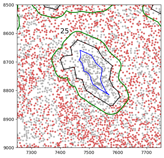
[36]:
import matplotlib.patheffects as PathEffects

markersize = 10

fig, ax = plt.subplots(figsize=(6, 6))

## all points
ax.scatter(
    *zip(*adata.obs[["X_centroid", "Y_centroid"]].to_numpy()),
    s=markersize,
    color="grey",
    alpha=0.5,
    label="All cells"
)

# Points in selected commnities
xy = adata.obs[
    adata.obs["SOX10+CCND1-"]
][  # [adata.obs[communitycolumn].isin(communityIndexList)][
    ["X_centroid", "Y_centroid"]
].to_numpy()
ax.scatter(
    xy[:, 0],
    xy[:, 1],
    s=markersize,
    color="r",
    marker="o",
    alpha=0.4,
    label="SOX10+CCND1- cells",
)

spc.plt.plotRegions(
    final_holes,
    colors_list=["black"],
    ax=ax,
    label_bounds=(6000, 6300, 9050, 10000),
    x_offset=5,
    y_offset=5,
    add_label=False,
)
spc.plt.plotRegions(shrunken_holes, colors_list=["blue"], ax=ax, add_label=False)
spc.plt.plotRegions(
    extended_holes, colors_list=["green"], ax=ax, add_label=False, linewidth=2
)
txt = plt.text(7400, 8600, "25", fontsize=16, color="black")
txt.set_path_effects([PathEffects.withStroke(linewidth=8, foreground="w")])
plt.ylim(8500, 9000)
plt.xlim(7250, 7750)
ax.invert_yaxis()
[37]:
def merge_pheno(row):
    if row["phenotype_large_cohort"] in [
        "T cells",
        "Cytotoxic T cells",
        "Exhausted T cells",
    ]:
        return "T cells"
    elif row["phenotype_large_cohort"] in ["Melanocytes"]:
        return "Tumor cells"
    else:
        return "Other cells"


# Applying the function to create the new column
adata.obs["pheno"] = pd.Categorical(adata.obs.apply(merge_pheno, axis=1))
[38]:
adata.obs.head()
[38]:
| X_centroid | Y_centroid | phenotype_large_cohort | id | CCND1_cellRingMask_positive | CCND1_negative | SOX10_cellRingMask_positive | SOX10+CCND1- | COI_community | region_rough | ... | hole_33 | hole_34 | hole_35 | hole_36 | hole_37 | hole_38 | hole_39 | hole_40 | hole_41 | pheno | |
|---|---|---|---|---|---|---|---|---|---|---|---|---|---|---|---|---|---|---|---|---|---|
| 0 | 21807.565909 | 9.997727 | Unknown | 0 | True | False | False | False | -2 | BG | ... | BG | BG | BG | BG | BG | BG | BG | BG | BG | Other cells |
| 1 | 21896.527273 | 28.150000 | Unknown | 1 | True | False | False | False | -2 | BG | ... | BG | BG | BG | BG | BG | BG | BG | BG | BG | Other cells |
| 2 | 21891.008824 | 31.755882 | Unknown | 2 | True | False | False | False | -2 | BG | ... | BG | BG | BG | BG | BG | BG | BG | BG | BG | Other cells |
| 3 | 21893.457692 | 37.430769 | Unknown | 3 | True | False | False | False | -2 | BG | ... | BG | BG | BG | BG | BG | BG | BG | BG | BG | Other cells |
| 4 | 21888.600000 | 35.496000 | Unknown | 4 | True | False | False | False | -2 | BG | ... | BG | BG | BG | BG | BG | BG | BG | BG | BG | Other cells |
5 rows × 53 columns
[39]:
regions = ["Tumor", "Tumor Border", "Stroma Border", "Stroma"]
macro_df = []
for r in regions:
    df = spc.measurements.getRegionComposition(
        adata, "pheno", regions=[r], regioncol="region_rough"
    )
    df["region"] = r
    macro_df.append(df)
df = spc.measurements.getRegionComposition(
    adata, "pheno", regions=regions, regioncol="region_rough"
)
df["region"] = "Overall"
macro_df.append(df)

macro_df = pd.concat(macro_df)
macro_df
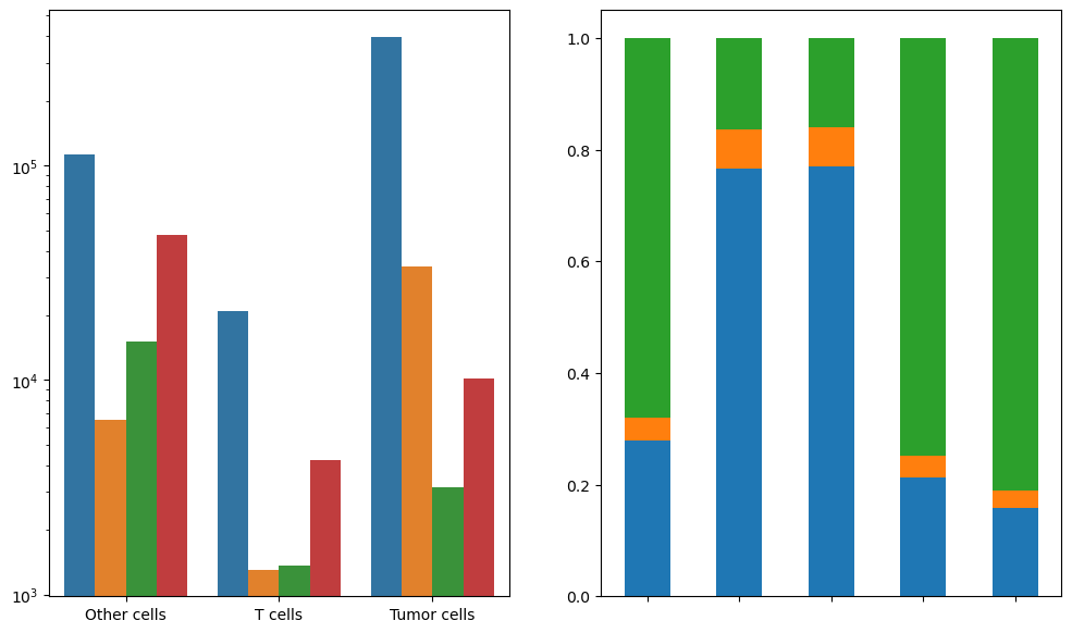
[39]:
| pheno | cell_count | composition | region | |
|---|---|---|---|---|
| 0 | Tumor cells | 398217 | 0.748067 | Tumor |
| 1 | Other cells | 113177 | 0.212608 | Tumor |
| 2 | T cells | 20934 | 0.039325 | Tumor |
| 0 | Tumor cells | 33720 | 0.811045 | Tumor Border |
| 1 | Other cells | 6551 | 0.157567 | Tumor Border |
| 2 | T cells | 1305 | 0.031388 | Tumor Border |
| 0 | Other cells | 15152 | 0.769919 | Stroma Border |
| 1 | Tumor cells | 3160 | 0.160569 | Stroma Border |
| 2 | T cells | 1368 | 0.069512 | Stroma Border |
| 0 | Other cells | 47571 | 0.767027 | Stroma |
| 1 | Tumor cells | 10199 | 0.164447 | Stroma |
| 2 | T cells | 4250 | 0.068526 | Stroma |
| 0 | Tumor cells | 445296 | 0.679215 | Overall |
| 1 | Other cells | 182451 | 0.278295 | Overall |
| 2 | T cells | 27857 | 0.042491 | Overall |
[40]:
fig, [ax1, ax2] = plt.subplots(1, 2, figsize=(12, 7))
macro_plot_df = macro_df.copy().drop(columns=["composition"])
macro_plot_df = macro_plot_df[macro_plot_df["region"] != "Overall"]

sns.barplot(
    data=macro_plot_df, ax=ax1, x="pheno", y="cell_count", hue="region", palette="tab10"
)
macro_plot_df = macro_df.copy().drop(columns=["cell_count"])
macro_plot_df2 = macro_plot_df.pivot(
    index="region", columns="pheno", values="composition"
)
macro_plot_df2.plot(
    kind="bar",
    stacked=True,
    legend=False,
    ax=ax2,
    color=["tab:blue", "tab:orange", "tab:green"],
)
plt.xticks(rotation=0)
ax1.set_ylabel("", fontsize=14)
ax1.set_xlabel("", fontsize=14)
ax2.set_ylabel("", fontsize=14)
ax2.set_xticklabels(["", "", "", "", ""])
ax2.set_xlabel("", fontsize=14)
ax1.get_legend().remove()
# ax2.legend(loc="lower left", markerscale=5, bbox_to_anchor=(1, 0.5))
ax1.set_yscale("log")
# plt.savefig("5_macro_region_composition_vert.png", dpi=300, bbox_inches='tight')
/Users/ghwan/opt/anaconda3/envs/spatialcells/lib/python3.10/site-packages/seaborn/categorical.py:253: FutureWarning: The default of observed=False is deprecated and will be changed to True in a future version of pandas. Pass observed=False to retain current behavior or observed=True to adopt the future default and silence this warning.
grouped_vals = vals.groupby(grouper)
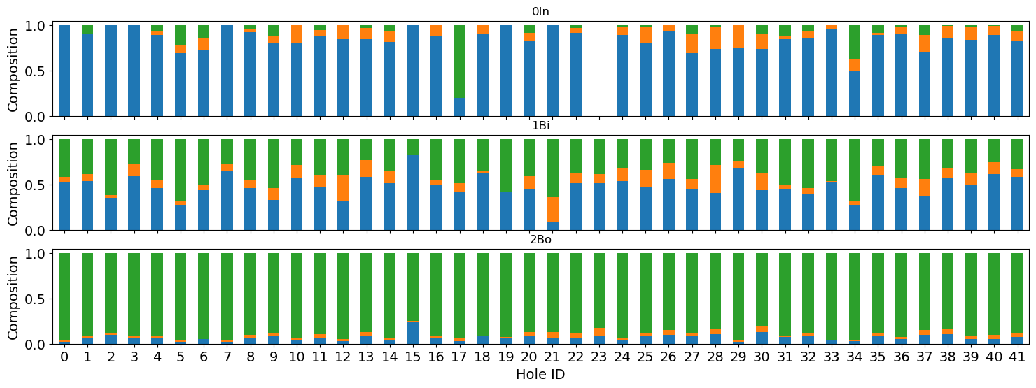
[41]:
micro_df = []
regions = ["0In", "1Bi", "2Bo"]
for i in range(len(final_holes)):
    for r in regions:
        df = spc.measurements.getRegionComposition(
            adata, "pheno", regions=[r], regioncol=f"hole_{i}"
        )
        df["region"] = r
        df["hole_id"] = i
        micro_df.append(df)
micro_df = pd.concat(micro_df)
micro_df
[41]:
| pheno | cell_count | composition | region | hole_id | |
|---|---|---|---|---|---|
| 0 | Other cells | 9 | 1.000000 | 0In | 0 |
| 1 | T cells | 0 | 0.000000 | 0In | 0 |
| 2 | Tumor cells | 0 | 0.000000 | 0In | 0 |
| 0 | Other cells | 86 | 0.530864 | 1Bi | 0 |
| 1 | Tumor cells | 67 | 0.413580 | 1Bi | 0 |
| ... | ... | ... | ... | ... | ... |
| 1 | Tumor cells | 36 | 0.327273 | 1Bi | 41 |
| 2 | T cells | 10 | 0.090909 | 1Bi | 41 |
| 0 | Tumor cells | 162 | 0.875676 | 2Bo | 41 |
| 1 | Other cells | 14 | 0.075676 | 2Bo | 41 |
| 2 | T cells | 9 | 0.048649 | 2Bo | 41 |
378 rows × 5 columns
[42]:
fig, axs = plt.subplots(3, 1, figsize=(6, 18), sharex=True, sharey=True)
micro_plot_df = micro_df.copy().drop(columns=["cell_count"])
for i, r in enumerate(micro_plot_df.region.unique()):
    tmp = micro_plot_df[micro_plot_df.region == r]
    tmp = tmp.pivot(index="hole_id", columns="pheno", values="composition")
    tmp.plot(
        kind="bar",
        stacked=True,
        figsize=(18, 6),
        legend=False,
        ax=axs[i],
        color=["tab:blue", "tab:orange", "tab:green"],
    )
    axs[i].set_title(r)
    plt.sca(axs[i])
    plt.xticks(fontsize=14, rotation=0)
    plt.yticks(fontsize=14)
    plt.ylabel("Composition", fontsize=14)
    plt.xlabel("Hole ID", fontsize=14)
    # plt.legend(loc="lower left", markerscale=5, bbox_to_anchor=(1, 0.5))
# micro_plot_df = micro_plot_df.pivot(index="region", columns="pheno", values="composition")
# micro_plot_df.plot(kind="bar", stacked=True, figsize=(6,6), legend=True, ax=ax1)
# plt.savefig("5_micro_region_composition.png", dpi=300)
